Topographic Corrections: Final Boss Edition

In a previous blog post, I talked about the many, many issues I’ve had with handling the complexity that is accurate modelling of the temperatures of planetary surfaces. This is mainly because, unlike their conception as perfect round spheres we display in elementary school classrooms, planets are bumpy. While changes in input required to model temperatures on the surface a perfectly smooth sphere (or ellipsoid) are easy enough to implement, accounting for this true bumpiness at a small-scale level is hard.[1]I should say medium-scale, as there are even more issues with modelling the effects of the roughness of planetary surfaces on human-foot-to-bacterium-size-scales, but that’s a topic for yet another time…

Thankfully, generations of Earth scientists before me (and even before any of this measuring-the-temperature-of-space-rocks nonsense) have known about this, since it, uh, affects our lives down here quite a lot. From 100 km up it may not seem to matter if a desert is flat or filled with tall rocks, but when it’s the difference between you standing in the shade of one or being blasted by UV on the open Sahara, you’d probably wanna know if they’re there. Furthermore, while I’m just trying to use this temperature modelling to figure out what rocks are made of beneath the surface of a dead world with no people on it, down on Earth an accurate knowledge of surface temperatures has a huge range of implications for all kinds of human activity—agriculture, weather forecasting, urban planning, water availability, civil engineering, and many, many other areas. The techniques to predict these temperatures have thus become quite sophisticated, especially since the invention of computers and the launch of Earth-orbiting satellites to monitor these conditions on a global scale.

It was in the rabbit hole of researching this vast and complex literature that I found several sources pointing back to one of the (seemingly) foundational papers on this topic: a paper from 1981 by Jeff Dozier and colleagues from the University of California, Santa Barbara, that described the calculation of horizons and skyview factors from digital elevation model (DEM) data in a more computationally efficient way that enabled it to actually be performed on a reasonable scale with the limited computing technology available then. Dozier followed this up with a 1990 paper with James Frew (also from UC Santa Barbara) that implemented these techniques in a way suitable to modern DEM grids, and it was off to the races! Together, these two papers have been cited over 800 times, and the techniques mentioned in them seemed to come up again and again in subsequent geography-based Earth system modelling papers.

While I’ve talked in the past about implementing the algorithms from Dozier and Frew (1990) before[2]including my “contributions” to the GitHub project topocalc which is a modernized python version of the code, it was recently while looking up the paper again for the umpteenth time that I discovered that in the fall of 2021, the very same Jeff Dozier from the 1990 paper finally published a follow-up that revised the methods for a modern computational environment, including the development of parallel processing and the use of geographic DEM grids (i.e. latitude-longitude, rather than the projected ones measured in fixed-length units like meters used in many other areas of Earth science focused on small-scale regions). That latter point is huge, since almost all planetary datasets are stored as an unprojected grid given in latitude-longitude points with a certain number of “pixels per degree” (ppd). There are both benefits and severe disadvantages to this type of data storage, since the spacing between grid points in this system is not uniform on spherical/ellipsoidal objects (see the many, many problems with trying to turn spheres into rectangles), but for better or worse it’s become standard in the delivery of planetary datasets.

It turns out, in addition to the theoretical considerations discussed in the paper, Dr. Dozier also published the MATLAB code that implements them. Since I’m finally in the academic system and have access to a MATLAB license again, this was fantastic! Let’s just download it and let ‘er rip!

…Well, not so fast. For one thing, almost all software built for manipulating DEMs like this assumes Earth-based coordinate systems, which have become quite standardized and are the default in many GIS-related programs. Thankfully, this code came with the option to input a custom ellipsoid model, but making sure that all of the MATLAB functions called within it didn’t make some sneaky Earth-centric calculation assumptions was critical and tedious to check. I also discovered, in the process of “tracing” the code’s many interdependent functions and scripts, that it had two major limitations: 1) even though it implemented geographic calculations to determine solar azimuth angles, distance spacing between grid points, and other important geometric considerations, it notably did not take into account the curvature of the Earth when doing the actual calculation of the horizons; and 2), it only performed nearest-neighbour interpolation to create the rotated grids along which the horizon calculation could be performed. To understand why these are (potentially) significant issues, let’s start with number 1:

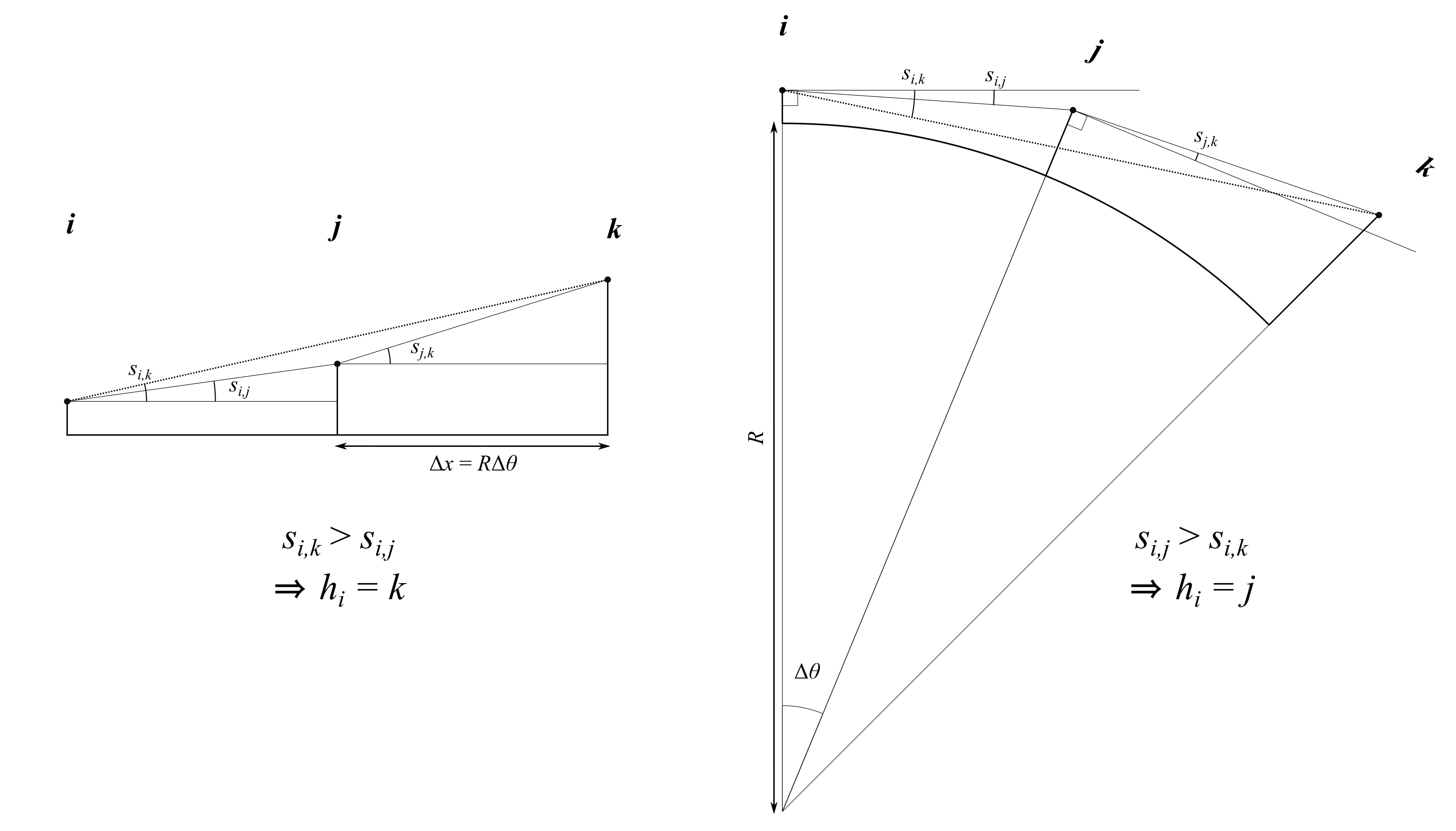
The horizon calculation works by passing in a line along a series of grid points, and calculating the angle between each of them. The maximum angle for a given point is called that point’s “horizon”, and describes the location of other features in the DEM (i.e. a mountain or a tall rock) that shade sunlight coming from that direction. On Earth, the assumption that these grid points essentially lie along a straight, flat line is a relatively good one-–-see the existence of Flat Earthers (and the surprising difficulty of actually observing the effects of Earth’s curvature) as an example. However, a well-known geometric fact (courtesy of, who else, Carl Friedrich Mother-Fucking Gauss) states that the curvature of a surface can be described by the radius of the circle that is tangent to it at a point; thus, more highly curved surfaces have a smaller radius of curvature, and conversely, the surfaces of planets with smaller radii will be more highly curved, as Le Petit Prince could easily tell you:

While not quite whimsically-tiny-asteroid-sized, the Moon is substantially smaller than the Earth, and thus its surface is more highly curved. The upshot of this is that objects which would otherwise have obscured a given point from the Sun on a (nearly-)flat surface are actually lower than expected on a curved surface, and this effect increases as you move further away. Since many of the small craters and impact melts I’m interested in modelling occur on the rims of much larger craters, calculating the actual height of the distant rims they’re contained within could be affected by this quite significantly.

Perturbed by this realization, I immediately spent an ungodly amount of effort and days on trying to derive the right formula to account for this curvature when calculating horizons. A colleague of mine, who was also interested in thermal modelling of the Moon (although not on quite such small, detailed scales), presented a relatively simple formula at a Diviner team meeting:

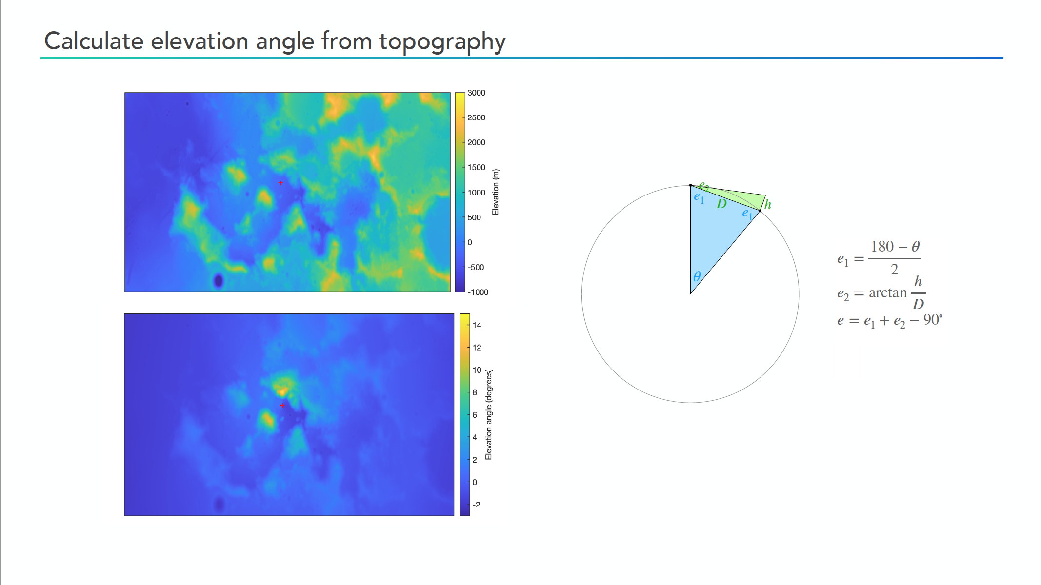
However, upon closer inspection this diagram and its associated computation makes several approximations that aren’t quite correct. The first is that the distance, D, is measured in a straight line from the observer to the point being observed: in reality, the distances are measured along the curved outer surface of the ellipsoid(/circle) rather than the chord passing between the two points. The second is that the height shown in the diagram is measured perpendicular to the chord between the observer and base of the DEM point, rather than the true direction parallel to the radius connecting the surface with the center of the object. These might only be minor corrections to the basic picture, but I couldn’t live with myself until I tested whether they would actually affect the resulting calculated horizons significantly.

After many sleepless nights and hopeless scribbling in circles of half-remembered high-school trigonometry, I finally stumbled upon (what else) a stack overflow thread of someone looking to implement a similar computation. I don’t know who you are or what you’re doing with your life now, Vivin Paliath, but G-d bless your little sketch of a diagram. With the right triangles in hand, it was finally simple to follow through the trigonometry and find the correct formula, which I re-drew in Inkscape and summarized in the figure below:

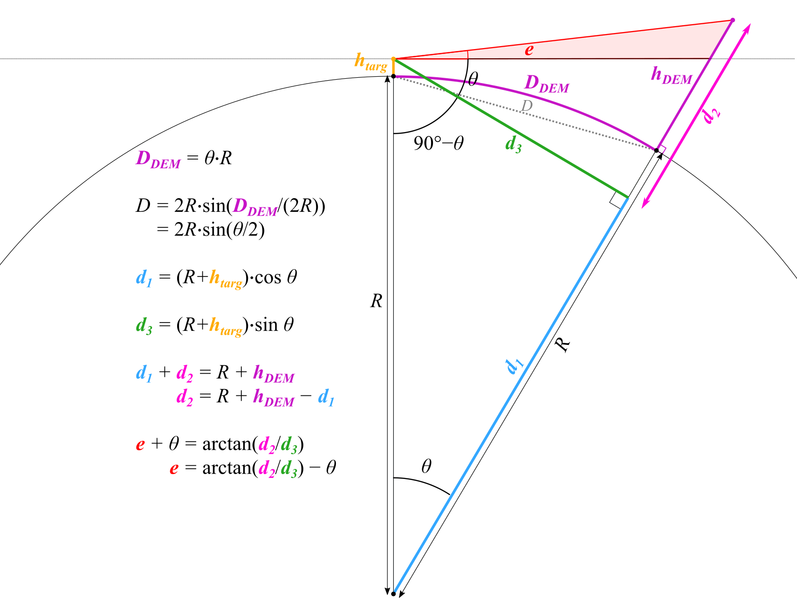
We can see with this diagram that we get the correct formula for the elevation angle, e, which is the same thing as the horizon angle when it is at a maximum for a given point in a given direction. One other notable aspect of this formula is that, unlike in the simplified flat model, it’s actually possible to have negative elevation angles/horizons if you happen to be on a very high spot of the planet looking out over lower-lying terrain. To compare back to Tyler’s formula, I found the same patch of the Moon as he showed above, ran my formula against his, anddddd (drumroll)…

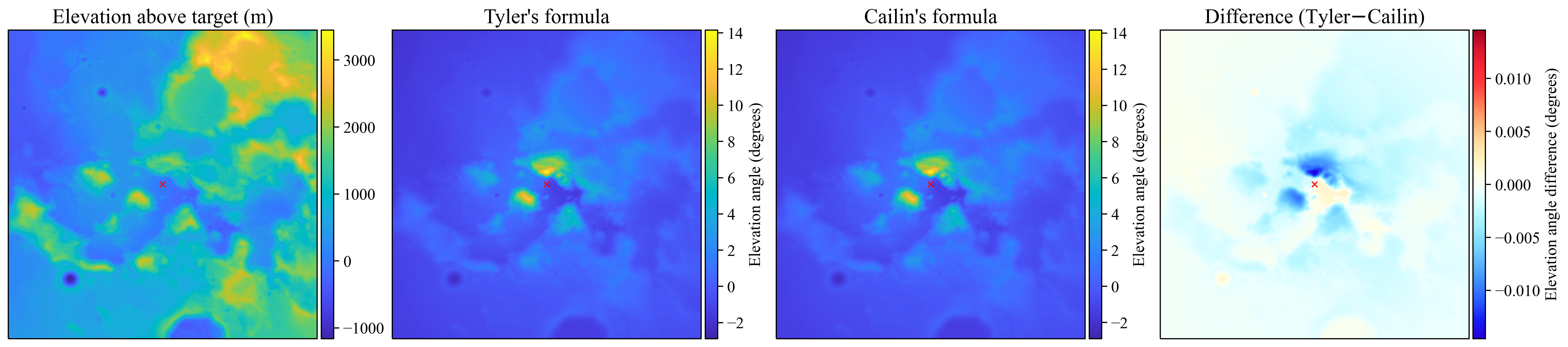
…Found <0.01 degrees of difference at maximum. Okay, so it turned out not to be such a big deal, but I’ve been working on this damn project for four years—when I finally publish, every single little piece of it is going to be as accurate as humanly possible, damn it!

Despite this minor difference, I still used my new formula when updating the 2021 MATLAB code from Dozier (remember him?). I had to do some other slight modifications to remove the restrictions of assumed-positive horizons, but it was relatively straightforward. And with that, I was off to the races! Right? …Right?

Okay, of course not—you knew I wouldn’t be writing an entire damn essay about this if it were that simple. It turns out another limitation of the Dozier code (and, in fact, many others that I examined) is that they all do nearest-neighbour interpolation to get the values of both the DEM when rotated to compute the horizon in a certain direction, and the lat/lon values of the corresponding points where the calculation is performed. This works… okay, especially for most Earth-based circumstances where the DEM data are very high-resolution and the sunrise/sunset location shifts enough due to the Earth’s seasonal cycle that high-precision calculations are the least of your worries. But the Moon has almost zero obliquity (i.e. tilt of its rotational axis relative to the ecliptic plane), and so the Sun rises in almost the same place all year round, especially near the equator. Thus, high-resolution horizons could be the difference between a relatively-good model input that can be fit adequately to nighttime data, and utter garbage that completely ruins the nonlinear least-squares fitting routine.

If the horizons are even slightly off, the model will predict massively different temperatures just before/after sunset than exist in reality due to the lack of an atmosphere on the Moon and its extremely slow rotation period, and thus the algorithm will frantically jerk the proverbial steering wheel to try to turn that predicted curve up (or down) enough to fit that data—see example above. This absolutely destroys the sensitivity to the relatively tiny, ~1 Kelvin difference in temperature produced from differences between buried impact melt and ordinary regolith, and results in Pollockian catastrophes like this when the final fit parameters are mapped:

The green part in the figure above is real and corresponds with where impact melt is seen in the high-resolution images, but all of the cyan-coloured stuff completely drowns out the signal and makes everything else look like a midwestern trans girl’s 2017 glitchwave album cover.

Getting these horizons right turned out to be… way more important than I had expected initially, and also, unfortunately, a huge pain. So, on to problem 2: interpolation.

The problem with naïvely using a form of interpolation other than nearest-neighbour (say, bilinear for example) is that the DEM heights, latitude grid, and longitude grid all have to be rotated the same way, but if you interpolate the lat/lon values you get nonsense near the edges. For example, if you use a value of 0 for the background fill of the new grid after rotation, and then interpolate a pixel halfway between this and a point on the edge of the longitude grid with a value of, say, 45°E, then the resultant longitude value would be 22.5°E—wayyyyy off from where it should be located. On the other hand, interpolating using nearest neighbour will mean you may lose some spatial points (up to 18% of them, in fact), and these will both be unable to influence the calculation of the horizon as well as needing to be filled in somehow when the grid is rotated back.

However, through the power of Math™, instead of interpolating between the original grid and a fill-in background value, I was able to compute the location in the original grid where the coordinates in the rotated grid came from using an inverse transformation, and then manually do the interpolation in the latitude and longitude directions separately, only retaining valid values. And amazingly… this worked! I could now rotate the DEM by any small amount I wanted, and the horizons would be accurately calculated based on interpolation between the available grid points. So, with trembling hands, I pushed the “run” button on my code to calculate all the horizons for a small crater area, and…

Success!

Even better than that, when you compare it to the original code I used which didn’t include curvature, you can visibly see the effect it has: the rim of the large crater far off to the west doesn’t create as high of a horizon as it would in the assumed-flat case:

Finally, just last night, I was able to bring all this together and put my new method to the true test: could it get rid of the garbage pixels that showed up in previous versions of the thermal model fitting algorithm? Well, I’m happy to report that…

…it can!!!

This version includes no penalty function to limit the parameters to a certain range, but it does include a statistical test that differentiates between whether a single-parameter or 2-parameter model is necessary to fit the data—hence why it doesn’t appear to be quite as sensitive to the melt area. However, selecting, implementing, and comparing model-selection and goodness-of-fit criteria like these is a huge topic that could easily fill an entire post of its own, so for now, it’ll have to wait for it’s own day in the Sun!

Till next time,

xoxo gossip grad