Analog Arcana
As I discussed in a previous post, electronics has been an on-again-off-again hobby of mine ever since a childhood friend introduced me to the world of passive solar-powered robotics almost two decades ago.[1]I mean, uhhhh, a few years ago. I’m definitely 23. While we did have to learn the basics of electric circuits (Ohm’s law, Kirchhoff’s voltage law, etc.) in high school physics, and I took undergrad classical E&M, there’s never really been a time where my scientific work has overlapped with needing to understand the specifics of how the electronic instruments that gather the data we use every day actually work.
So imagine my surprise when I stumbled across this video recently:
This is from a 2011(!!!) talk by Michael Scarito at DEFCON, a hacker convention held annually in Las Vegas, Nevada. Scarito goes through a brief rundown of the principles of radar and what it can be used for, before delving into a project (originally spearheaded by Dr. Greg Charvat of MIT) to build a handheld-sized radar system using off-the-shelf components and a couple of coffee cans (no, seriously). We’ll come back to this near the end, since I think it illuminates a number of rather complex elements of a typical radar system, but first: a narcissistic detour![2]Listen, I have to keep something about this blog gay.
Although I’ve barely dipped my toes into the waters of radar theory (and certainly haven’t dedicated enough time to actually working through the physics of polarimetry and dielectric interactions), my background in electronics has made me want to truly understand the technology behind it from the ground up. Building radio circuits has long been a distant goal of mine—the closest I got was a crystal radio kit (much like this one) when I was 11, and even then it seemed like arcane magic to be able to summon the sound of the human voice from thin air with just a few passive components.

While I haven’t been very good on following through on that ambition in a practical sense, I’ve still been fascinated by radio technology and its long and winding history. One of the first resources that caught my attention was this video by Technology Connections on the “superheterodyne” radio. What on[3](or off) Earth does that name even mean!? It turns out, though the technology was invented literally over a century ago, it still forms the backbone of all modern radio systems—and, yes, even radar!
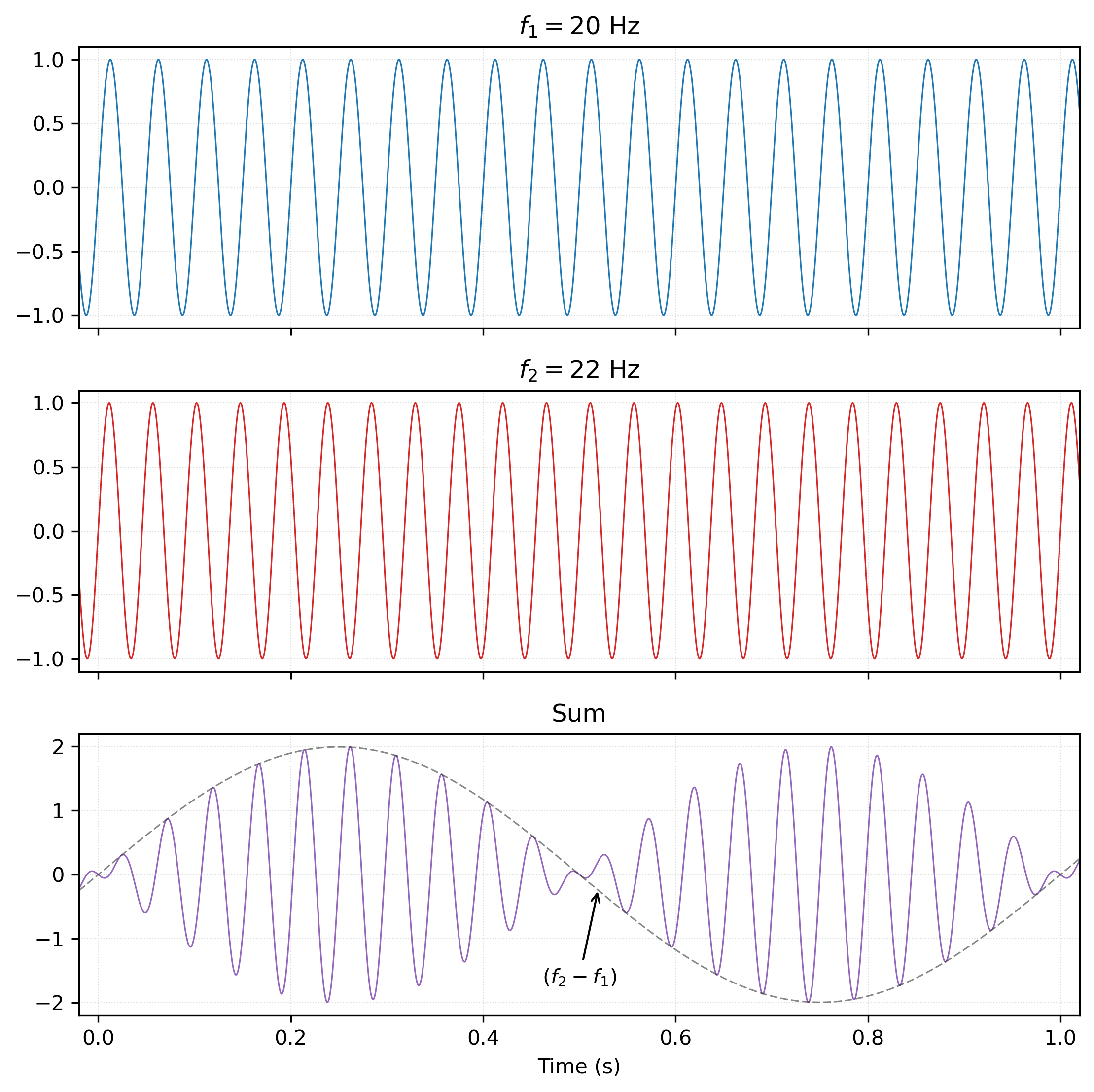
The fundamental principle of the heterodyne (we’ll leave out the “super” part for now) is that if you want to tune a receiver to a certain radio frequency, you don’t actually have to build a moveable filter to select out that frequency. You see, radio waves, like all electromagnetic waves, behave like, well, waves, and thus all of the weird and wonderful phenomena seen in other wave mechanics apply to them as well. If you happen to play a stringed musical instrument, you may even have practical experience with some of these properties. Ever had to tune a guitar and used the harmonics on the 5th and 7th frets to listen for the “warbling” to slow down until they’re in tune? (If you have no idea what I’m talking about, here’s a video[4]Warning: incoming guitar-dude-droning-on-unnecessarily-long.)
The “warbling” is what’s referred to as “beating” in acoustics, and it results from the peculiar alternation of constructive and destructive interference when adding two sine waves with very similar (but not identical) frequencies. As you can see below, the resulting “beat frequency” (the frequency of the amplitude envelope of their sum), is simply the difference between the two input frequencies.[5]Technically, there’s also another component produced that is the sum of the two frequencies (f1+f2) rather than their difference, but for our purposes this doesn’t matter and is generally filtered out in practical applications.
So what does this have to do with radio? Well, the unfortunate thing about electrical circuits is that they are never ideal, and the combination of parasitic capacitances and inductances and other fun messy real-world garbage they produce means they have a limited ability to react to fast-changing signals. Unfortunately for us, radio waves can be very fast-changing signals—AM radio, for example, uses frequencies of 540 to 1600 kilohertz (for reference, the maximum frequency human ears can hear is typically about 20 kHz). FM frequencies are even higher: 88 to 108 megahertz. If we tried to select a band of these fast-changing electrical signals directly using a filter, they’d just get smeared out into a slightly wiggly but basically constant voltage.
But fear not! It’s (super)heterodyne to the rescue! A superheterodyne radio uses the exact same principle of beat frequencies discussed above to convert the extremely high frequency of the radio signal into a usable signal at a lower frequency that can be filtered with precision. The reason this works is that, normally, the desired information to be transmitted (e.g. audio, video, etc.) isn’t encoded directly into the wave at the radio frequency itself; rather, some type of modulation is used on a carrier frequency, encoding information in the changing of that parameter of the carrier wave (incidentally, this is the reason for the names AM and FM radio, for the two main types of modulation used to send audio signals: Amplitude Modulation and Frequency Modulation). Since the carrier itself is not important, only the changes to it over time, we can safely use a superheterodyne to lower the carrier frequency while preserving all the important information. The “super” in “superheterodyne” just refers to the fact that this carrier wave is in the ultrasonic frequency range above normal human hearing.
But wait: in the guitar string example, we had two sine waves vibrating at the same time to produce the interference—where does the second one come from here? Well, that’s the genius of a superheterodyne: it creates its own, local, tuneable oscillating signal, and then injects this into the mixer to produce a constant beat frequency that is then filtered out by the radio’s circuitry![6]The original idea of a “heterodyne”, or “difference in frequencies”, was invented by Canadian Reginald Fessenden in 1901, by transmitting both carrier signals at the same time and mixing them at the receiver end. The superheterodyne, on the other hand, has slightly more disputed origins, as it was independently discovered and patented by three separate people in three countries between 1917 and 1920 The following block diagram demonstrates what’s happening fairly well:

The tuneable oscillator produces a signal that is used to both filter the incoming signal (to only select the difference of the two frequencies, rather than their sum) and to be injected into the mixer to produce the beat frequency. Several amplifiers ensure the received signal has enough power to be worked with adequately, and then the signals are mixed and then filtered at the constant filter frequency. The demodulator then extracts the encoded audio information, which sends it to an audio amplifier, then a speaker, and—hey presto! That’s radio, baby.
The journey to understanding radio circuits became even more fascinating when I discovered this series from a team of engineers working to restore the communications system used on the Apollo missions:
Notably, by the time of Apollo, NASA needed a radio that could deliver voice, television, telemetry, tracking, and ranging all in one compact system. Previous spacecraft had used separate radio signals for these and a C-band (4-8 GHz) passive beacon received by ground stations for tracking, but at the Moon the distances would be too great for such a tactic; thus, a combined active transmission and ranging system was required.
If you have time, I strongly encourage you to watch the above series, as it delves into way more depth than I have time or space to cover here. The major takeaway, though, was that this was the first time S-band radio transmissions were used on a spacecraft. The S-band covers the range of 2-4 GHz, and for Apollo the S-band system was locked on a very precise carrier frequency near 2.1 GHz. But wait… where have I seen that frequency range used before…

Mini-RF!?
Yep, that’s right: the standard frequencies used in planetary radar today are (at least partially) a result of the development of radio frequency standards for Apollo. Another interesting fact is that if we convert the S-band frequencies into wavelength, we get the standard ~12 cm that Mini-RF uses—right in the middle of the microwave range.
So with all of that context, let’s finally return to the video that started this post. How exactly do we turn a radio, which just has to send/receive and decode a signal, into an instrument that can image a planetary surface? The trick is to take advantage of ranging (the time delay between the transmission of a signal the receiving of its reflection) and the Doppler effect (the shift in frequency of a wave due to the line-of-sight motion of its emitter/reflector). If we pulse a radio signal, we can measure the time it takes for the transmitted pulses to be reflected off of a surface and return to the receiver; thus we can determine the range to an object by converting this timing to distance using the speed of light, c, as long as the pulses are transmitted with enough spacing for all of the reflections to return before we start the next one.
What about the lateral spacing? For a rotating body, we can take advantage that one side is rotating towards the observer, while the other side is rotating away; thus, the Doppler effect will shift the reflected frequencies from one side of the body vs. the other (actually, depending on our frequency sampling we can get a range of different distances across the body). This figure from my supervisor’s chapter in the Encyclopedia of the Solar System explains it fairly well:

There’s one final complication, however: if we just transmit a signal with a constant frequency, how will we know which delays are associated with which Doppler shifts? And, furthermore, if the round-trip time of the radar beam is (relatively) long (e.g. ~2.5 s for the round-trip to the Moon and back from the Earth), how can we build up enough data fast enough to actually produce an image?
The answer is to use a chirp. Instead of using a constant frequency, if we instead ramp up the frequency with time, then we can differentiate different pulse arrivals by their start frequency, and their Doppler shifts by the (coherent) shift of the chirp across the entire received signal. (I think there’s a bit more nuance to this, but I have to watch the talk again to fully understand it.) Here’s a graph of what a typical chirp looks like:

So that’s it! By stacking and identifying each received pulse, we can produce a time series that allows us to then obtain a 2D plot of the received delay times and the Doppler shifts.
Finally, let’s return to the talk from the beginning of the post. The intervening 50 years since Apollo have seen the rise of WiFi in order to keep us all tethered to our universal hand-held anxiety machines wherever we go, and WiFi came to adopt 2.4 GHz and 5 GHz as its standard operating frequencies. Because this is also in the microwave radar range, there are suddenly a ton of low-cost microwave radio components available to the average consumer. Thus, for (at most) a couple hundred bucks, one can build a fairly sophisticated radar system that can be carried in a person’s hands:

We can see all of the fundamental components here: the chirp (/ramp) generator, the tuneable oscillator (the voltage-controlled oscillator or VCO), several signal amplifiers, and the mixer that performs the superheterodyne magic. And, as promised: cantennas! The one thing I forgot to mention was that the radio signal in a radar needs to be focused in one direction in order to prevent reflections from all other surfaces around it, and it just so happens that metallic-coated coffee cans do the trick perfectly (well okay, maybe there could be some improvements with professional antenna design, but still—clever!)
Overall, getting deeper into this world has really given me an appreciation for how technologies and concepts that seem like arcane magic at first can actually be understood by mere mortals with a little work. And beyond that, it’s even more empowering that one can not only understand these technologies, but also even build them due to the increasing availability of inexpensive electronic components. I haven’t achieved my radio-construction dreams as of yet, but with all this knowledge under my belt, maybe that’ll be the next step before I make the jump to the even more state-of-the-art in radar theory and electronics that I’ll need for my PhD research.
Till next time,
-xoxo gossip grad ☾⋆⁺₊⋆