Over the past few years I’ve struggled on and off with my PhD work, sometimes hitting months-long stretches where I hardly get anything done at all and can barely stand to look at my computer. You might find this hard to believe, given how much I can babble on about my research whenever someone has the temerity to ask, but truth be told these last four years have been punctuated with some of the lowest points in my entire life. While the details of those abyssal episodes may eventually make it into another blog post, in this one I’d like to talk about a little self-care practice that’s been an invaluable reminder of why I decided to pursue this work in the first place.
Everyone loves pictures from space—when the James Webb Space Telescope released its first science images in July of 2022, the amount of social media attention was overwhelming. The venerable Astronomy Picture of the Day, which has been posting every day since 1996(!), is a frequent source of screensavers and backgrounds for space aficionados. Personally, this highly-oblique image of the surface of Europa, taken from the Galileo orbiter in 1997, was one of the most influential in setting me down the path of studying planetary science:
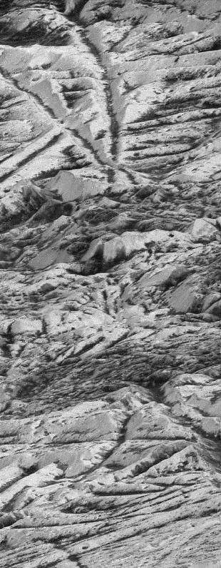
The view at the center of this image is just under 2 km wide, meaning that the vertical topography is only 10s to 100s of meters high—gently rolling hills and valleys whizzing past the window on a cosmic cross-continental flight. You can almost imagine skiing or hiking this terrain, the faint Sun off to one side of the black, airless sky, and the greating, shining hulk of Jupiter in another. Images like these were some of the first times I felt like the moons and planets of our solar system were real places, physical locations that felt as tangible as the Scarborough Bluffs that I climbed in my youth. And it is the oblique perspective, replicating what you might see on a spaceship flying over these fantastic alien landscapes, that really brings them to life.
Of course, for most scientific work, these images are not ideal to work with. Scientists generally prefer views with a consistent scale throughout the two-dimensional image plane, as these are far easier to interpret and map-project onto other datasets to derive useful insights. But aside from their aesthetic value, oblique images can sometimes provide useful scientific information as well: pairs of such images taken from opposite vantage points can produce very accurate topographic suface maps through stereo processing, or quantitative data on how light scatters off a surface in different directions.
LRO
The Lunar Reconnaissance Orbiter’s twin high-resolution Narrow-Angle Cameras (NAC) are an example of such nominally nadir-pointing cameras that are sometimes used for so-called “off-nadir” imaging. However, this isn’t quite as simple as point-and-shoot photography like the Apollo astronauts acquired with their Hasselblads out the window of the Command Module—the NACs are “pushbroom” imagers, meaning that their sensors are very wide and high-resolution in the direction perpendicular to the spacecraft’s nominal motion (the “cross-track” direction), but have only a few dozen rows of pixels in the in-track direction.
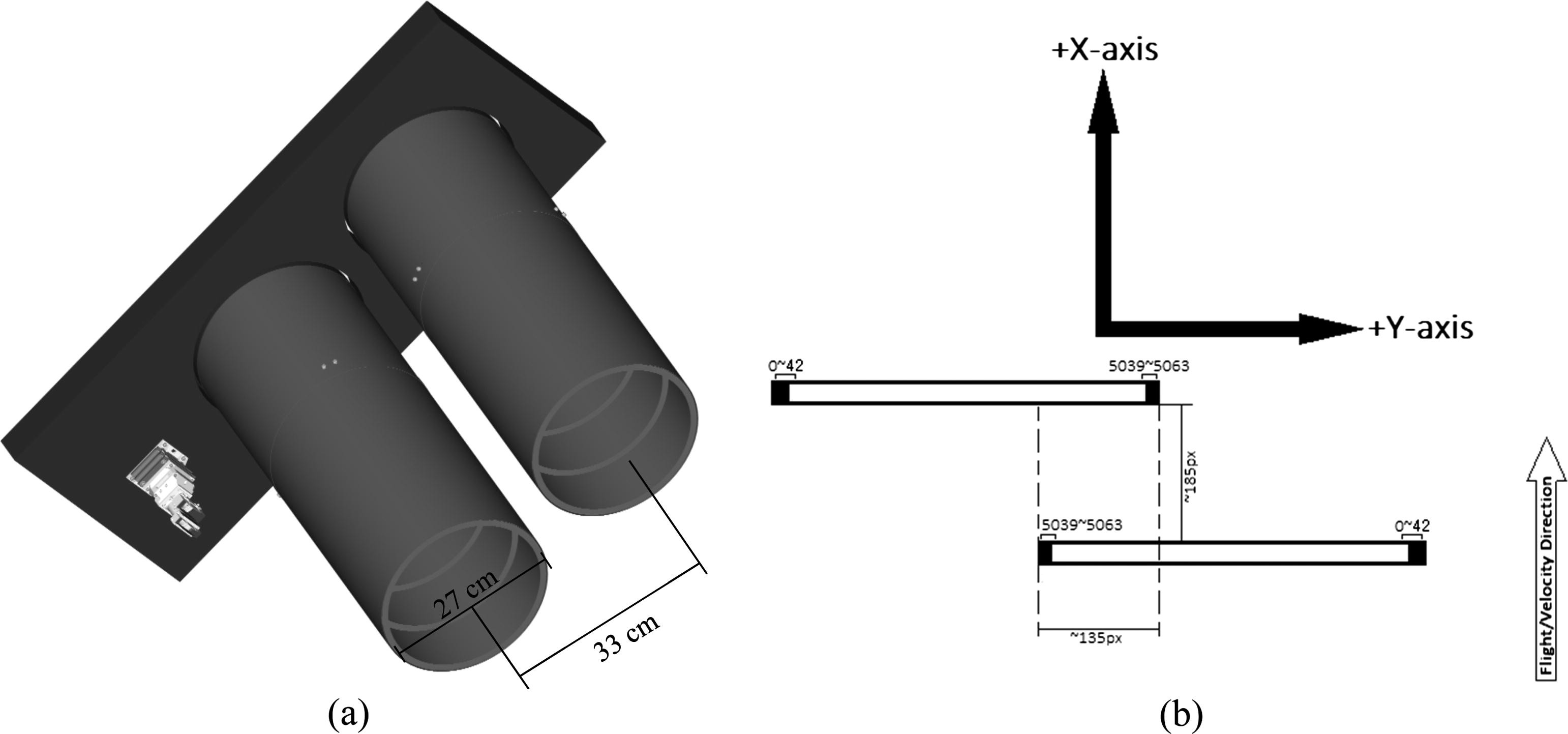
Because LRO orbits at close to a constant velocity, this configuration is ideal for collecting long strips of data when the cameras are pointed straight downward, achieving very high resolutions (down to <30 cm/pixel!) while still covering a significant portion of the surface.
A second issue is that the NAC cameras are bolted onto the body of LRO in a fixed orientation, meaning that in order to take an oblique image, the entire spacecraft must roll over onto its side—this, of course, requires the use of either reaction wheels or small thrusters to achieve reorientation, both of which have a limited lifespan due to either mechanical failure or fuel exhaustion.[1]In fact, in 2018 one of the instruments used to control LRO’s orientation—the intertial measurement unit (IMU)—was powered off due to degradation from the space radiation environment, leaving it with only the star-tracking cameras for geometric orientation. This would have severely limited the ability of the spacecraft to perform off-nadir slews, as the cameras must be unocculted by the Earth, Moon, or Sun (including sunlight glare) in order to accurately determine LRO’s position. Fortunately, a new algorithm that automatically calculates a slew path to avoid any of these obstacles has brought the spacecraft back to full performance, and with current fuel estimates LRO will probably be operational to the end of the 2020s and possibly even into the 2030s.
With these caveats in mind, it’s no wonder that there are relatively few oblique images released on the LROC website. However, when digging through the raw NAC archives to generate the image mosaic for Korolev Z in my recent paper, I accidentally stumbled upon an oblique view I had never seen before:
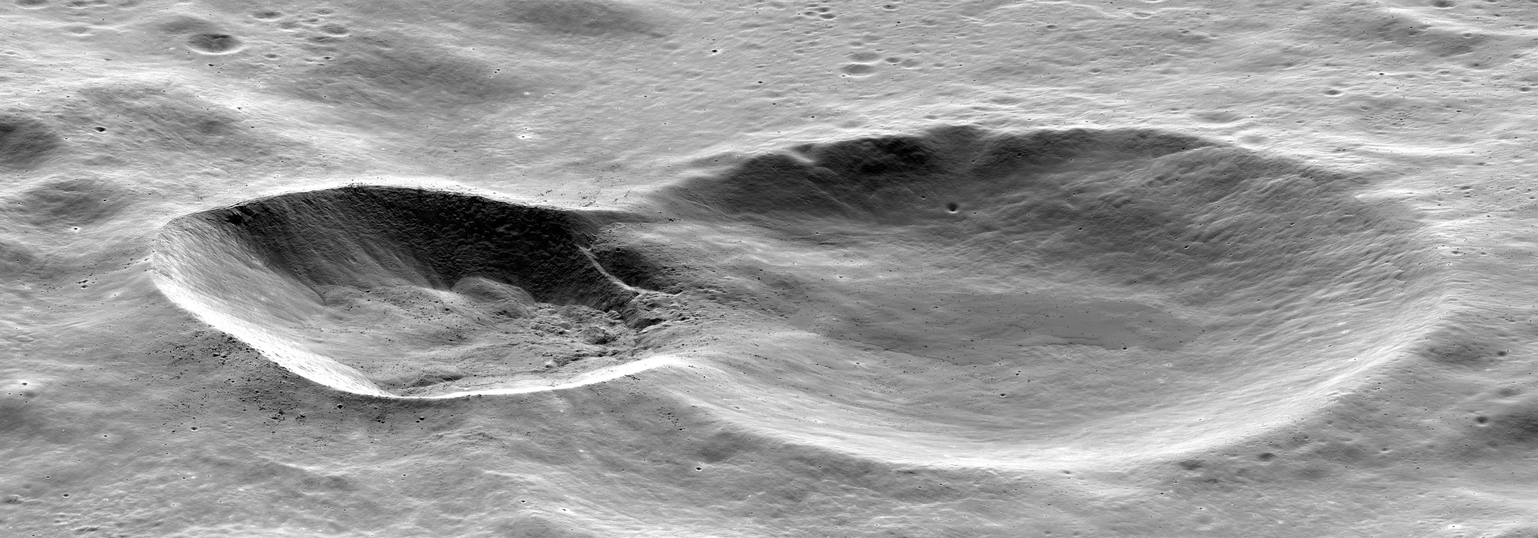
The version uploaded here is 3x-downsampled, but at full resolution the amount of detail is incredible: individual boulders sticking up out of the impressive impact melt flow that spilled over into Korolev X are visible, back-lit by the Sun in this extremely high-phase (~114°) image. What does this mean? A diagram may help clarify things:
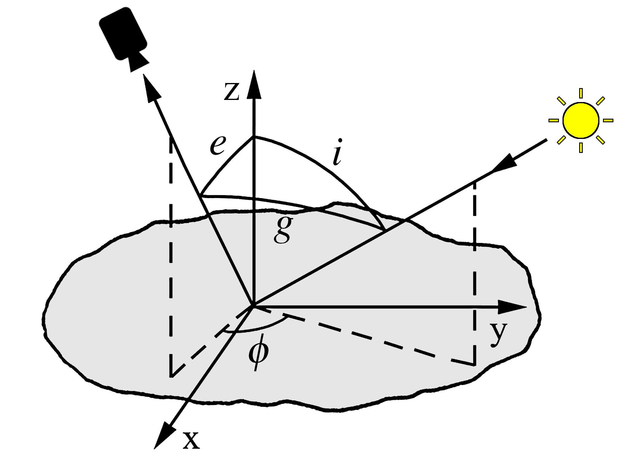
Planetary observations can be described by several geometric parameters relating the relative positions of the spacecraft, illumination source, and the surface under observation using polar coordinates. The angle from the normal of the surface[2]the vector perpendicular to the local “flat” tangent plane, equivalent to the $z$-axis in the above diagram to the illumination source is called the incidence angle ($i$); similarly, the angle from the surface normal to the observing spacecraft is called the emission angle ($e$). The angle between the incidence and emission angles can be described in two ways: either the azimuth angle around the pole of the surface normal ($\phi$), or simply the direct angle in 3D space—this is what is known as the phase angle ($g$).[3]In radar/radio astronomy, this is also known as the bistatic angle, because of course radio scientists just have to be different 🙄[4]Okay okay fine it actually is for a good reason: the term “phase” as used to describe the spatial alignment in the peaks and troughs of electromagnetic waves is a much more important concept in radar systems than most other ranges of the EM spectrum, since here the wavelengths are large enough that relative phases between transmitted and reflected waves are significant and can usually be directly measured. This leads directly to the concepts of polarimetric and interferometric radar, which can provide a substantial amount of information about the physical properties and relative movement of the target(s) under observation.
This helps explain why high-phase images are both beautiful and rare in planetary imagery: they create an ethereal, otherwordly glowing effect on surfaces or atmospheres viewed from these angles, but they can also potentially fry instrument sensors if they catch a direct glimpse of the Sun.[5]A famous example of this was the accidental Sun-viewing that fried the television camera on Apollo 12, a mistake which astronaut Alan Bean reflected on with some embarrassment several years later. They are also uncommon in orbital instruments because these are usually designed to be nadir-pointing, which guarantees the highest spatial resolution possible and makes georeferencing and geodetic control of the data much more straightforward. The most frequent place these types of images are encountered in planetary datasets are during flyby missions as the spacecraft look back on their object of study towards the Sun, exemplified in stunning photos such as New Horizons’ view of Pluto’s backlit mountains and atmospheric hazes or Cassini capturing plumes of water ice erupting out of geysers in the south pole of Saturn’s moon Enceladus. Here, the missions only have one[6]Or sometimes a few, in the case moon flybys by spacecraft orbiting their host gas giant planets shot to get their data, so every image counts, and high-phase images can be especially important for studying atmospheric structures on those bodies that have them.
This rarity is all the more reason why I think it’s a shame the high-phase LROC images are not more widely known or seen by the public. It is therefore in the spirit of helping others see these marvellous photographs (and bring future ones to light) that I present my workflow for creating them from publicly-accessible data using open-source tools.
Typical NAC Processing
In generating the dozens of image mosaics of the various craters used in my research, I’ve now developed quite a streamlined pipeline for going from raw NAC data to finished map-projected products. Here’s a general overview of my process:
- Find LROC NAC frames covering the target area by creating a box in Quickmap and searching for NAC products (optional: constrain by observation angle, including by emission angle if you want to find oblique images)
- Download the raw EDR frames from the LROC website (from both the left and right camera)
- Use the USGS’s ISIS software to prepare, calibrate, and map-project the frames onto a shape model of the Moon[7]Note that this file provides elevations relative to the lunar reference radius (1737.4 km); to use this as a shapefile in ISIS you will need to first convert it to use absolute radius values
I’ve made available here a Bash script that will execute the ISIS commands for all the image data in the folder where it’s run (note that you first need to have a working copy of ISIS installed). Let’s step through these commands one by one and see what they’re doing:
for i in *.IMG; do

    lev0file="${i/.IMG/_lev0.cub}"
This loops through every raw .IMG binary file in the current folder, creating a new file with the name [old_file_name]_lev0.cub.[8]Note that this is how all the subsequent files are renamed, so I’ll leave out this step in the following descriptions. Next we actually get to the ISIS processing steps:
    lronac2isis from="$i" to="$lev0file"
    spiceinit from="$lev0file" web=yes shape=user model=/path/to/dems/Lunar_LRO_LOLAKaguya_DEMmerge/Lunar_LRO_LOLAKaguya_DEMmerge_60N60S_512ppd_radius.cub
These are two of the most important commands; lronac2isis ingests the binary file and converts it into the “cube” format used in ISIS. spiceinit then takes this file and attaches the relevant SPICE information, which consists of tables of navigation, timing, and instrument calibration data that are used for proper camera modelling and instrument geometry/photometry processing. This is also where information about the planetary body the instrument is targeting is added, which is why I referenced a user-defined shape model in this step.
    lronaccal from="$lev0file" to="$lev1file"
    lronacecho from="$lev1file" to="$lev1echofile"
These two commands apply NAC-specific photometric and instrument corrections.
cam2map from="$lev1echofile" to="$lev2file" map=MoonEquirectangular180.map pixres=map
This is where the majority of the heavy lifting is done. cam2map uses a model of the LROC NAC cameras plus the attached SPICE information to project the original rectangular array of pixels onto the surface model. In most cases with nadir-pointing geometry, this won’t result in noticeable distortion of the image, but the resulting output file will now have pixel locations that correspond to accurate latitude-longitude coordinates on the surface.[9]Well, relatively accurate, anyway—there are usually slight variations between the modelled and real pointing of the camera, due to a combination of factors (unaccounted-for thermal expansion, imperfect SPICE data, etc.). The proper way to correct for this is to register the image to some known datum such as a global DEM, and then (for mosaics) use bundle adjustment to co-register a set of images with overlapping regions. See this LPSC abstract (warning: PDF) for a high-level discussion and an example of the improvements achieved with these techniques.
Oblique Tweaks
Here’s where the fun begins.
Unfortunately, the process for producing oblique images is not quite as easy to automate. The initial steps are largely the same as normal nadir processing, but instead of projecting the images onto a DEM surface,[10]Thus “mappifying” them in a way that would attempt to rubber-sheet them over the surface; for an example of what that would look like, click here we want to simply align the left and right images in camera-plane space to produce a full, rectilinear view of our target.
After producing the calibrated Level 1 frames, we can use the ISIS command qview to view them. This launches a graphical interface from which you can open the two files and place them side-by-side.
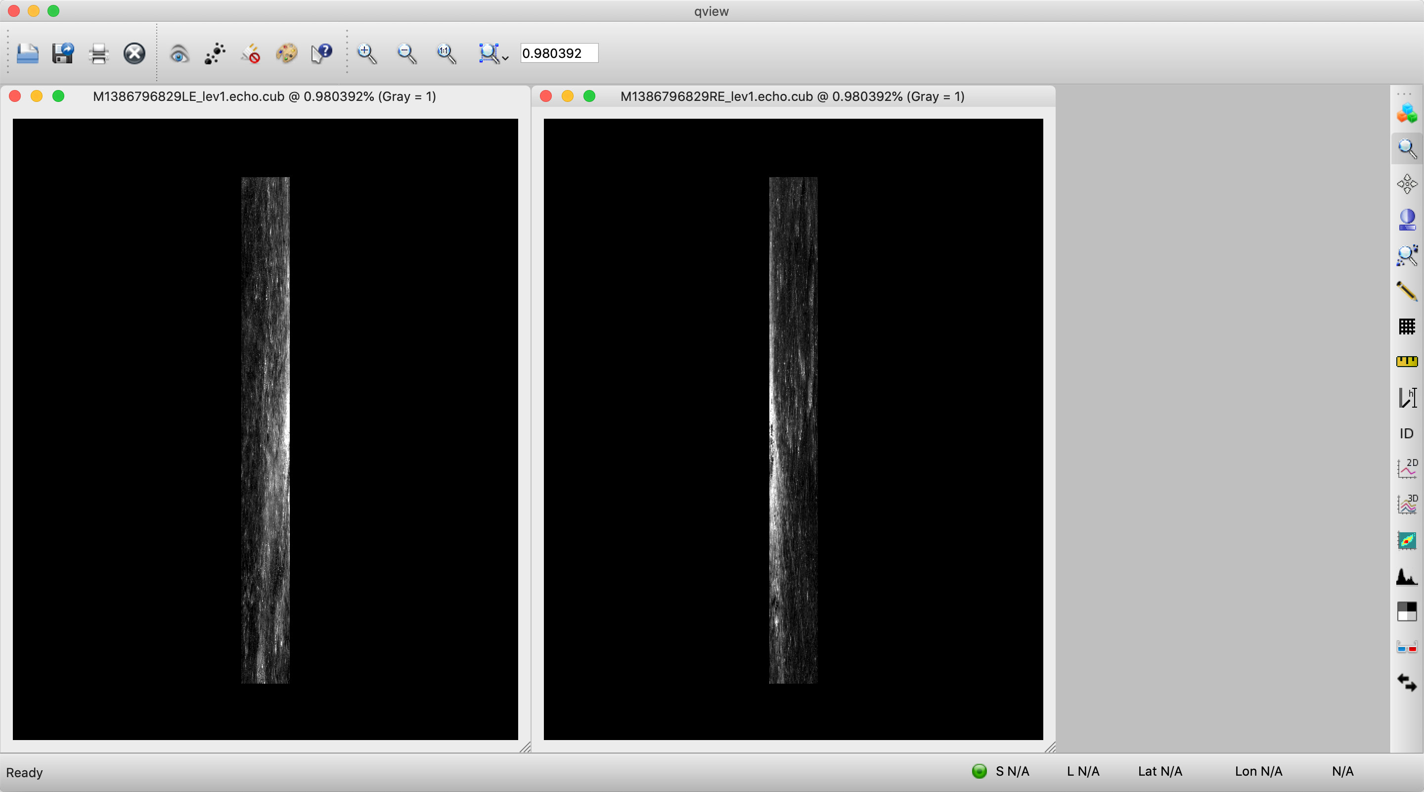
Our next task is to identify a matching feature in each of the left and right frames, which we will use to align them. While the L/R cameras are fixed in place and theoretically should always have the same orientation relative to one another, temperature changes in the spacecraft and the cameras themselves can cause them to slightly shift, so unfortunately a single offset value (as implied in the Wu and Liu (2017) figure above) won’t work for all images. In this case, I zoomed in on a region near the top of each image and found a bright crater with relatively sharply-defined features:
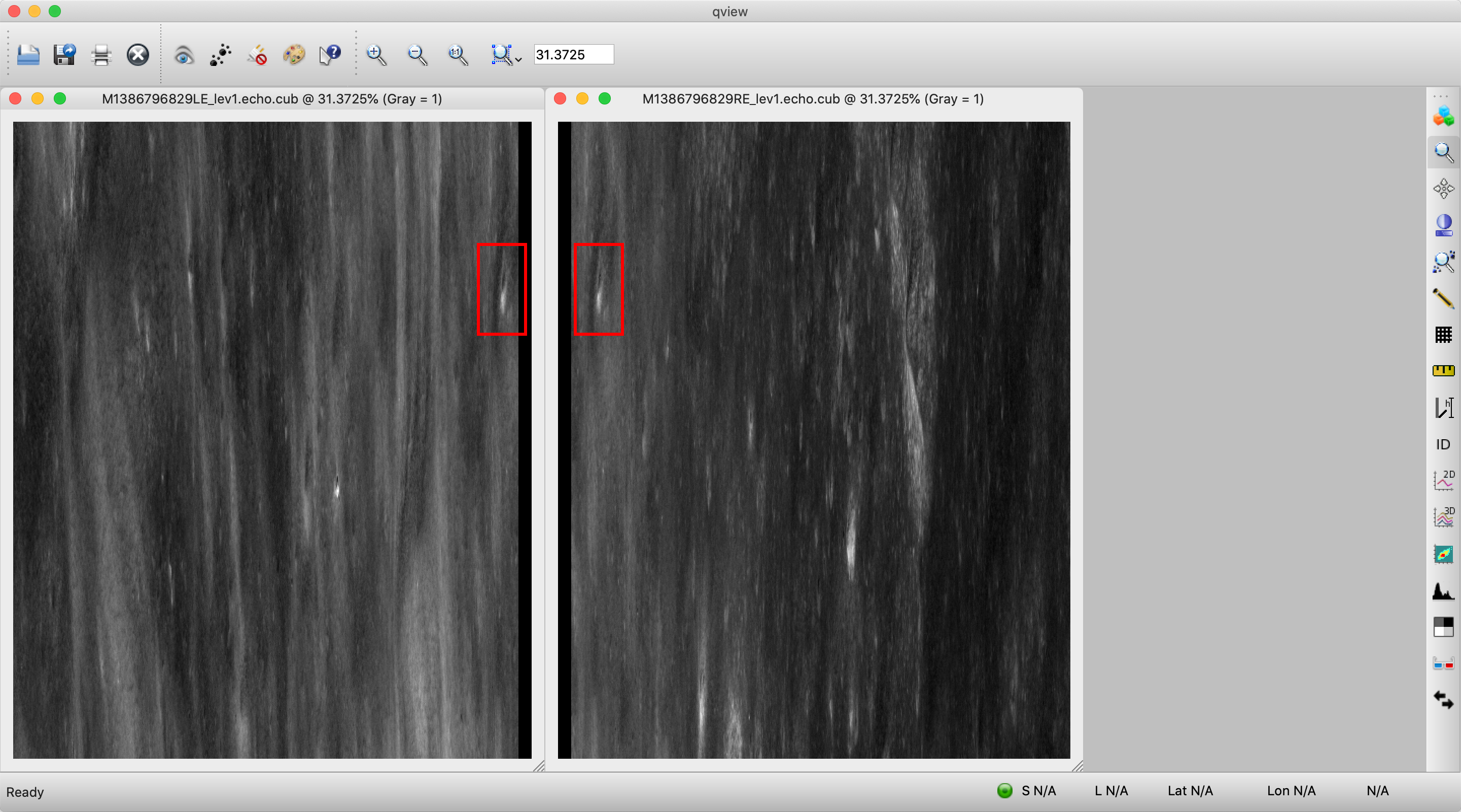
The contrast stretch of the images can be adjusted using the top toolbar (magenta outline) to make it easier to identify corresponding pixels (red pluses indicating mouse position; note that the window for each image needs to be clicked on/active to display the correct pixel coordinates):
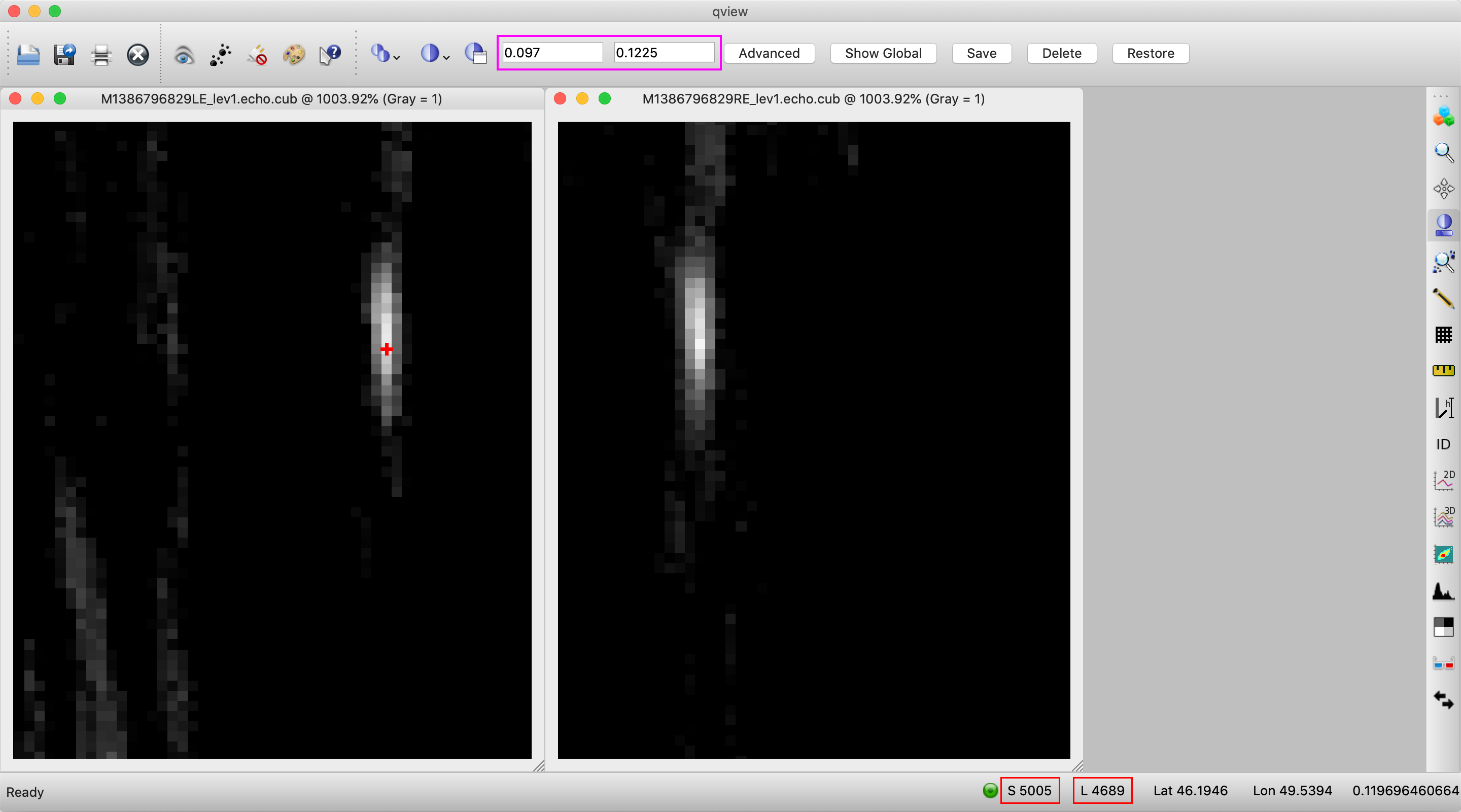
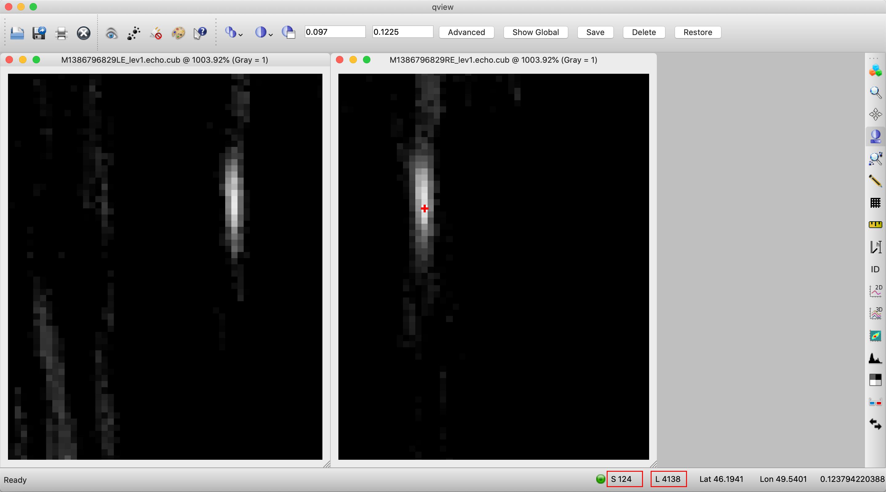
Note down the sample/line numbers of the corresponding pixels for each image (highlighted in red boxes at the bottom). We can then use these pixel positions to get the offset between the two images, simply by subtracting. In this case, the sample offset is 5005 − 124 = 4882, and the line offset is 4689 - 4138 = 551.
Next, we need to create the mosaic that will contain our two frames. To ensure we don’t cut off any part of the image, we will make its width equal to 2× an individual NAC frame, or 10128 pixels. For the height, we will use the length of a single NAC image (52224 pixels).[11]Although the two frames will have a vertical offset and thus their correctly-arranged height will be greater than one frame, the most they can possibly overlap is a single frame height, so we’re safe using this value. The syntax for this step is:
handmos from=M1386796829L_lev1.echo.cub mosaic=M1386796829LR.cub create=yes nlines=52224 nsamples=10128 nbands=1
Note that we use the create=yes keyword in this step to construct the image and place the left frame in it at the same time. Next, we use the offsets we obtained above to place the right frame:
handmos from=M1386796829R_lev1.echo.cub mosaic=M1386796829LR.cub outsample=4882 outline=551
This is where a particular quirk of the LRO spacecraft can rear its head: twice an (Earth) year, LRO performs a “yaw flip” maneuver to keep its single side-mounted solar panel correctly oriented towards the Sun. This is in fact a common procedure for Sun-synchronous satellites, as demonstrated in this animation of the NASA/CNES Jason-2 satellite:
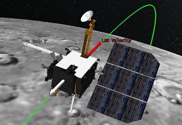
However, because of the pushbroom nature of the NAC cameras, these maneuvers actually reverse the orientation in which the pixels are read out as LRO scans over the surface, leading some images to be mirrored relative to their real-life perspective. This also means that the vertical offset of the two frames will be flipped, and thus the right frame will actually have a negative line offset relative to the left frame if we follow the procedure above. To check whether the frames are inverted, you can look on its WMS browse page, where there is a field for “LRO flight direction”; if this is “+X”, no action needs to be taken, but if this is “-X”, we will need to vertically flip the frames before mosaicking them:
flip from=M*L_lev1.cub to=M*L_lev1_flip.cub
flip from=M*R_lev1.cub to=M*R_lev1_flip.cub
After this, the steps are the same as above. At this stage, we could rotate our image to the correct (portrait) orientation using an ISIS command:
rotate from=M1386796829LR.cub to=M1386796829LR_rot.cub degrees=90 interp=nearestneighbor
However, even with nearest-neighbour interpolation this will actually resample the entire image and transfer the associated SPICE data to the new pixel coordinates, resulting in a very long processing time even for a simple 90-degree rotation. If you want to inspect your results, go ahead and do this; otherwise, we’ll forge ahead and complete the rotation later (at output), which can be done much more quickly once in a standard image format.[12]Note that if you do decide to rotate your image during this step, you will need to modify the script presented in the next paragraph to account for the swapped axes
Another annoying consequence of the pushbroom design of the NACs and LRO’s evolving orbit is that individual NAC pixels are not inherently square, and in fact depend on the spacecraft’s velocity at the time of acquisition. In the normal processing pipeline, this is not an issue, since performing map-projection on the frames inherently converts them into a representation with a fixed resolution specified in the map file. However, since we are working with the un-projected frames, we must manually calculate this approximate aspect ratio, and then apply a reduction that squishes the image into the approximately-correct dimensions. A script that I wrote derived from the one in this processing guide by the LROC team (warning: PDF) is used to obtain an approximation of this aspect ratio. To use it, you run it from the command line and supply it with the two level 0 (or level 1) frames:
./get_image_resolution.sh M1386796829L_lev0.cub M1386796829R_lev0.cub
It will then print the individual line/sample resolution for the center of each frame, their average, and finally the derived s_factor and l_factor for scaling the final assembled mosaic[13]Note that, in general, both the sample and line dimensions are scaled down for reasons not entirely clear to me but which seem to work out correctly. You could divide the two to obtain a scaling to apply only in the sample direction, thus preserving the maximum vertical resolution, but I was just following what was in that PDF guide.[14]Note also that the use of non-integer values in the scaling factors means there will be some resampling in the final image, but this should be worth the tradeoff of having approximately correct dimensions
reduce from=M1386796829LR.cub to=M1386796829LR_aspect_scale.cub sscale=3.753951083027643 lscale=1.2756094146789607
Outputting pretty pics
After all this ISIS processing, we can finally export our assembled oblique frame to a common image format for sharing with the world. ISIS provides support for outputting to a number of common file formats through the isis2std command, which also lets you set a number of output options depending on the file type. For our example, we will be outputting to JPEG, since we are mainly interested in creating pretty pictures and not preserving exact pixel intensity values.[15]Our image is also unprojected, since we only did level 1 processing—for non-oblique images, you would typically want to project them into a geographic coordinate system, as dicussed above. In these cases, outputting to a standard file with isis2std also creates a world file (e.g., .tfw for TIFF images) with geographic information, allowing the image to be imported into standard GIS software. A good overview of ISIS output options is available here
The first step in outputting is to return to qview and select a stretch that best captures the features in our image. Although the Moon is relatively uniformly low-albedo,[16]on average, it’s about as bright as a typical asphalt road! the ejecta of young impact craters can be significantly brighter, creating issues where they appear blown-out if the exposure range is set to produce a reasonable contrast level in the background terrain. Adjusting this is much more easily accomplished in typical image-editing software, so for now we mainly want to ensure we don’t lose detail when outputting from ISIS cube to JPEG format.
In qview, click on the
Next, we need to rotate the image to correct viewing orientation, as mentioned previously. In JPEG format, we can do this without modification of the actual image pixels by resetting and editing its EXIF data. We will need one additional tool for this procedure: the free exiftool developed by Phil Harvey. Once installed, we can issue this command to erase the EXIF data from our JPEG file:
exiftool -Orientation= -o M1386796829LR_aspect_scale_noexif.jpg M1386796829LR_aspect_scale.jpg
(Note the output file name comes first (after the -o tag), and the input file is at the end.) Now, if working on a Mac or Linux system, we can use a built-in tool called jpegtran to rotate the image and re-supply new EXIF data:
jpegtran -rotate 270 -outfile M1386796829LR_aspect_scale.jpg M1386796829LR_aspect_scale_noexif.jpg
Depending on the Z-axis orientation mentioned above, you may need to rotate the image either 90 degrees or 270 degrees to obtain the correct up-is-up orientation—if you mess up on the first try, just re-run the isis2std output command above, and try again starting from the exiftool step.
And voilà, the result! (Click to embiggenate)
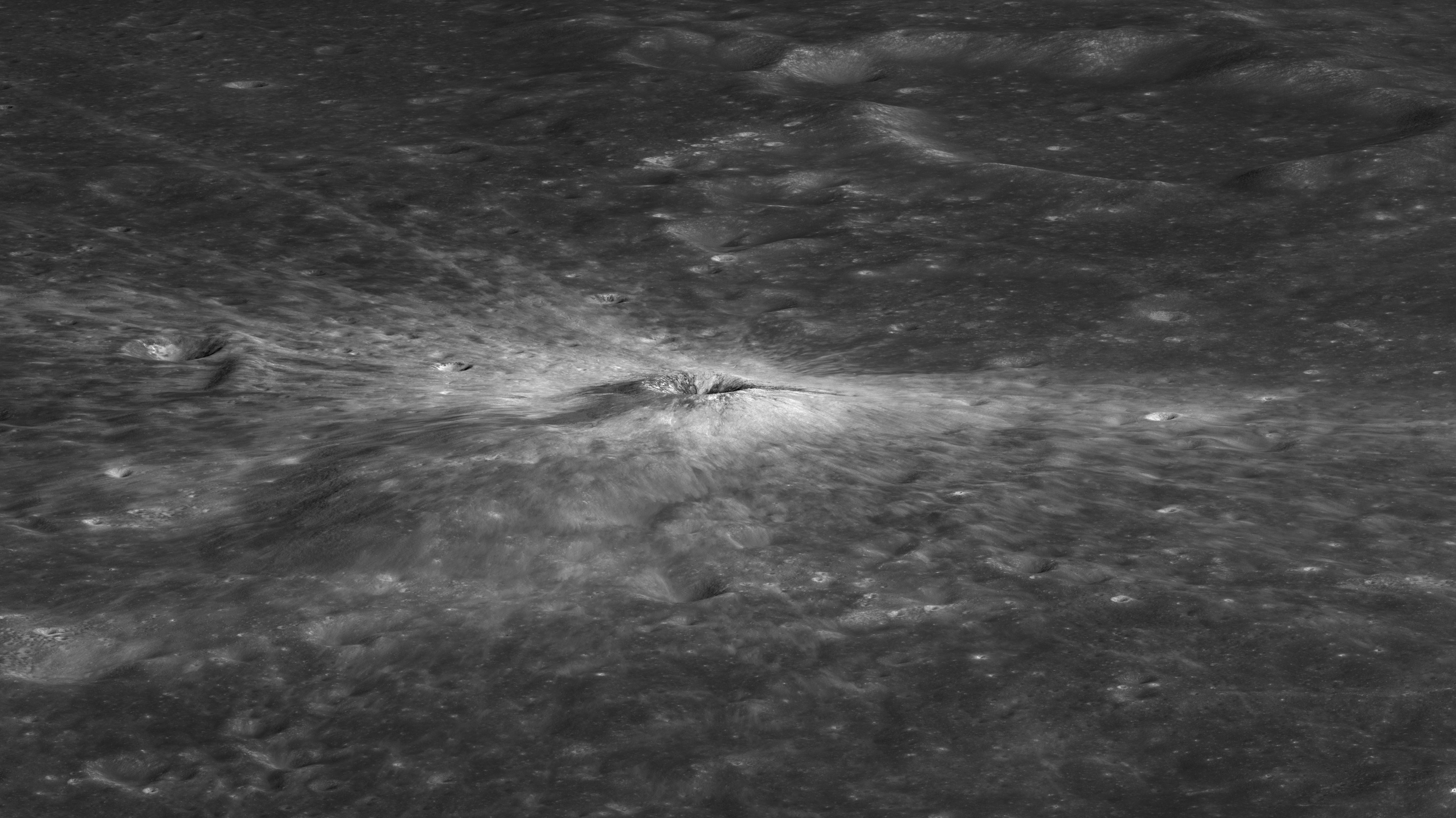
At this point, we’re basically finished. The final JPEG image will usually be a few tens of MB in size, and you may want to scale it down or import it into your favourite image editing software to adjust value curves and the like. For my images, I usually decreased their resolution by 4x to make them manageable for uploading on this website, but you can find the full-resolution versions on my Flickr.
%## Final thoughts
Till next time,
-xoxo gossip grad ☾⋆⁺₊⋆